Tutorial - Solving the six-hump camelback function

Filename: test/C6.py

The following tutorial shows how to find the global minimum of a Six-hump camelback function using the DIRECT algorithm.

\[ \begin{align}\begin{aligned}f(x_1, x_2) = (4 - 2.1 x_1^2 + x_1^4 + x_1^4/3) x_1^2 + x_1 x_2 + (-4 + 4 x_2^2) x_2^2,\\\Omega = [-3, 3] \times [-2, 2].\end{aligned}\end{align} \]

First we need to import the solve function from the DIRECT package:

>>> from scipydirect import minimize

Then we need to define the objective of the function:

>>> def obj(x):
  ...     """Six-hump camelback function"""
  ...     x1 = x[0]
  ...     x2 = x[1]
  ...     f = (4 - 2.1*(x1*x1) + (x1*x1*x1*x1)/3.0)*(x1*x1) + x1*x2 + (-4 + 4*(x2*x2))*(x2*x2)
  ...     return f

We need to define the domain of the problem using block constraints:

>>> bounds = [(-3, 3), (-2, 2)]

We use the DIRECT algorithm to solve the optimization problem. The algoritm is called using the minimize function. The solve functions accepts the problem objective obj and block constraints:

>>> res = minimize(obj, bounds)

In the above we use the default settings of the DIRECT algorithm. It us possible to costumize the algorithm using the parameters of the minimize function (see scipydirect.minimize()).

The minimize function returns a result object res making accessible the optimal point, res.x, the value of the objective at the optimum, res.fun, and a status message res.ierror.

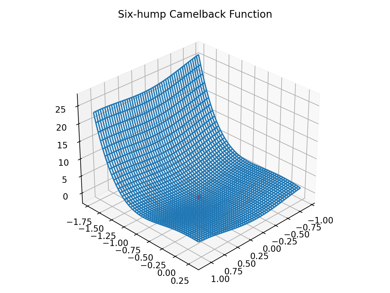
We can visualize the problem using matplotlib:

>>> fig = plt.figure()
>>> ax = fig.add_subplot(111, projection='3d')

>>> x = res.x
>>> X, Y = np.mgrid[x[0]-1:x[0]+1:50j, x[1]-1:x[1]+1:50j]
>>> Z = np.zeros_like(X)

>>> for i in range(X.size):
  ...     Z.ravel()[i] = obj([X.flatten()[i], Y.flatten()[i]])

>>> ax.plot_wireframe(X, Y, Z, rstride=1, cstride=1, cmap=cm.jet)
>>> ax.scatter(x[0], x[1], res.fun, c='r', marker='o')
>>> ax.set_title('Six-hump Camelback Function')
>>> ax.view_init(30, 45)
>>> plt.show()

This results in

(Source code, png, hires.png, pdf)

More examples can be found in the source distribution under the test/ folder.